Mixing and Blending: Using Residence Time Distribution to Understand Continuous Blending

In recent years, continuous powder mixing has attracted pharmaceutical processing, which has traditionally been a batch-based industry. However, while continuous processing is widely used in bulk solids manufacturing, especially for processing large material volumes in industries such as minerals, foods, detergents, and construction materials, few studies have been published on continuous bulk solids mixing^1-4.

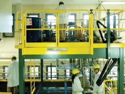
The most common type of continuous blender is the convective tubular blender, as shown in Figure 1. The convective tubular blender consists of a stationary horizontal mixing cylinder with a material inlet at one end and a material outlet at the other end. An overflow weir is typically mounted inside the cylinder before the material outlet to control the holdup of material within the blender. The cylinder contains a rotating shaft with impellers (such as blades, paddles, or ribbons) that mix the material by convection (moving the particles within the cylinder relative to each other). 

In operation, unmixed ingredients enter the blender’s inlet and are lifted, tumbled, sheared, and conveyed by the rotating impellers to the blender’s outlet, where the material exits the blender as a homogeneous stream. During steady-state operation, the mass flowrate into the blender equals the mass flowrate out of the blender, and the mass of material inside the blender (called the mass holdup) remains constant. 

Continuous Mixing Modes 

Material mixing within a tubular blender can be divided into two modes: cross-sectional (or radial) mixing and axial mixing. In Figure 1, for example, as two ingredients (Ingredient A and Ingredient B) are fed into the blender, we can consider them to be completely unmixed at the blender inlet, as shown in the cross section on the left in the figure. As the blender’s impellers rotate, they lift and tumble the ingredients, mixing the material in the cross-sectional plane. At steady state, cross-sectional mixing can be largely time independent, which means that each cross section in the blender exhibits the same arrangement of ingredients over time. As the figure shows, however, subsequent cross sections exhibit different ingredient arrangements. This is because when the impellers lift and tumble the material in the cross-sectional plane, some particles are pushed forward (and to a lesser extent, backward) in the cylinder, resulting in axial mixing as the material is transported and mixed along the cylinder’s axis.

Residence Time Distribution 

When material enters the blender during steady-state operation, most particles remain in the blender for a time close to a certain mean value, defined as the mean residence time. You can calculate the mean residence time by dividing the mass holdup by the mass flowrate. However, some particles experience faster convection in the forward axial direction, while other particles experience an unusual amount of backward pushing or occupy a “dead” volume within the blender for some time. This causes some particles to exit the blender very quickly, while other particles spend an unusually long time in the cylinder. As a result, a representative group of particles passing through a blender operating at steady state will have a range of residence times, called a residence time distribution (RTD). 

There are two idealizations of residence time behavior: plug flow and continuous stirred-tank flow. In plug flow, all particles move at the same speed along the cylinder’s axis, so particles entering the blender together exit the blender together and only cross-sectional mixing occurs. Continuous stirred-tank flow, on the other hand, assumes that particles entering the blender inlet are instantly and completely mixed into the rest of the material in the blender, so some particles exit instantaneously, while other particles take a very long time to exit. In reality, all blenders operate somewhere between these two idealized states. 

As will be discussed shortly, it’s possible to tune a blender’s RTD by changing certain operating and design parameters. The question is: what is a desirable RTD? For pure mixing applications, plug flow tends to be undesirable because accurately feeding bulk solid materials can be challenging. Feeders often directly precede blenders in the process train, and all feeders introduce a certain degree of variability. Feeders must also be periodically refilled, which can introduce sizable perturbations (also called noise) into the ingredient blend⁵. This noise will pass unfiltered through a blender operating in complete plug flow, which can affect the quality of the final product. 

For example, Figure 2a shows the concentration profile for one ingredient in a blend over time, after each unit operation in a tableting process train. The process train includes the ingredient feeders, a mill, a blender, and a tablet press, in that order. The ingredient concentration in the feed stream is indicated by the dark blue line, and the application’s maximum acceptable ingredient concentration is indicated by the horizontal purple line. The green line indicates a perturbation (a 0.25-gram pulse) in the ingredient concentration introduced into the feed stream that passed unfiltered through the mill. As indicated by the red line, the mixing that occurred in the blender dampened the effects of the perturbation enough that the ingredient concentration in the tablets (indicated by the turquoise line) remained below the maximum acceptable value. Note that this example’s RTD standard deviation value (a measure of the blender’s noise-filtering ability) is 12 seconds. If a 1-gram pulse (instead of a 0.25-gram pulse) of the same ingredient is introduced into the feed stream, as shown in Figure 2b, a blender operating at the same RTD and standard deviation value won’t be able to dampen the effects of the perturbation enough to keep the ingredient concentration in the tablets below the maximum acceptable value. 

However, if the RTD is widened to a standard deviation value of 24.9 seconds, as shown in Figure 2c, the blender can successfully dampen the larger ingredient pulse. Widening the RTD means that the blender is operating closer to continuous stirred tank flow, which allows the blender to filter the noise in the ingredient feed and maintain the quality of the final product.

Measuring RTD

Determining a blender’s RTD is critical to understanding and characterizing the blender’s operation. The RTD helps you understand how material flows through the blender as well as how effectively the blender will filter incoming noise from the unit operation immediately upstream. Determining the blender’s RTD also enables you to develop feed-forward (downstream) and feed-back (upstream) control strategies to ensure the final product’s quality. If you have incoming noise from a feeder or unit operation directly upstream, you can use the blender’s RTD to predict the composition of the blender’s output stream. You can then take feed-forward action to either reject out-of-spec product or take corrective action in downstream unit operations to bring the product back within specifications. You can also take feed-back action to eliminate the source of the noise. 

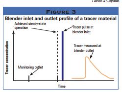
A blender’s RTD can be measured by introducing an instantaneous pulse of a tracer material into the material stream and measuring the tracer concentration at the blender’s outlet as a function of time, as shown in Figure 3. As the figure shows, the sharp pulse at the feeder inlet is broadened at the outlet due to axial convection as the tracer moves through the blender.

The mean centered variance (MCV) is the variance (square of the standard deviation) normalized by the square of the mean value of the distribution. In this case, the mean value of the distribution is the mean residence time. Standard deviation and MCV are qualitatively similar; both are a measure of the width of the RTD. 

Alternately, the tracer can also be introduced as a step function (an instantaneous change in the tracer concentration at the blender inlet). The system response (the tracer concentration at the blender outlet) would then be measured as a function of time and would depend on the blender’s RTD. 

Tracer Selection 

Using a tracer to measure a unit operation’s RTD is widely practiced, but the importance of selecting an appropriate tracer material is often overlooked. The tracer must have flow properties as similar as possible to the overall blend but must also be chemically distinguishable from the rest of the material. The tracer must not disturb the material stream’s flow behavior and should travel through the blender at the same rate as the rest of the material. 

Figure 4a shows a blender’s RTD when the physical properties of the tracer and the blend were similar. The overall throughput was 20 kilograms per hour (kg/h), and the impeller speed was 350 rpm. As the figure shows, the tracer material was fully flushed from the system within 10 minutes. However, the same blender under identical processing conditions exhibited a very different RTD when using a tracer material with a much higher bulk density than the blend. As shown in Figure 4b, the tracer had not fully exited the blender after 30 minutes of operation, resulting in incorrect RTD characterization. 

Adjusting RTD 

As previously mentioned, you can often adjust or tune a blender to achieve the desired RTD for your application. Changing the blender’s impeller speed is a common way to manipulate the RTD. Increasing the impeller speed decreases the mass holdup but also results in an increased MCV. For example, two RTD values for pure semi-fine acetaminophen running through a blender at 18 kg/h in steady state are shown in Figure 5. The tracer material was caffeine, introduced as a pulse at the blender inlet. The RTD on the left in the figure was obtained with the impeller speed at 350 rpm, while the RTD on the right was obtained with the impeller speed at 400 rpm. The disparity between the RTD shapes is discernible in the figure; operating at higher rpm results in a larger MCV value (0.406 at 350 rpm and 0.483 at 400 rpm). 

An alternate strategy for changing a material’s RTD is to manipulate blender design variables. This can be achieved by altering the blender’s incline angle or the angle of the weir at the blender’s outlet, but the RTD is most commonly adjusted by changing the impeller blade orientation⁶. Many blenders are available with adjustable impeller blades that you can orient to either push the material fully forward or backward or at an intermediate angle to manipulate axial mixing. Increasing the number of blades pushing material backward will generate an RTD with a larger MCV.

The total mass flowrate through the blender also affects the material’s RTD. Changing the overall mass flowrate to manipulate the RTD is uncommon, however, since mass flowrate changes imply an unsteady continuous process, and the mass flowrate of a process is generally predetermined based on production requirements and other nontechnical considerations. 

A blender’s RTD is a critical measurable attribute that aids in the understanding and design of a blending operation⁷. While the effects of process and design parameters and operating conditions on a blender’s RTD have been well examined, the effects of material properties on a continuous blender’s RTD remain largely unexplored. 

References 

1. Colin F. Harwood, Kenneth Walanski, Erdmann Luebcke, and Carl Swanstrom, “The performance of continuous mixers for dry powders,” Powder Technology, Vol. 11, No. 3, pages 289-296. 

2. Ralf Weinekötter and Lothar Reh, “Continuous mixing of fine particles,” Particle & Particle Systems Characterization, Vol. 12, No. 1, pages 46-53. 

3. B. Laurent and J. Bridgwater, “Continuous mixing of solids,” Chemical Engineering & Technology, Vol. 23, No. 1, pages 16-18. 

4. Sarang Oka, Abhishek Sahay, Wei Meng, and Fernando J. Muzzio, “Diminished segregation in continuous powder mixing,” Powder Technology, Vol. 309, pages 79-88. 

5. William E. Engisch and Fernando J. Muzzio, “Feedrate deviations caused by hopper refill of loss-in-weight feeders,” Powder Technology, Vol. 283, pages 389-400. 

6. Aditya U. Vanarase and Fernando J. Muzzio, “Effect of operating conditions and design parameters in a continuous powder mixer,” Powder Technology, Vol. 208, No. 1, pages 26-36. 

7. Sarang S. Oka, M. Sebastian Escotet-Espinoza, Ravendra Singh, James V. Scicolone, Douglas B. Hausner, Marianthi Ierapetritou, and Fernando J. Muzzio, “Design of an Integrated Continuous Manufacturing System,” chapter in Continuous Manufacturing of Pharmaceuticals, Edited by Peter Kleinebudde, Johannes Khinast, and Jukka Rantanen, Wiley-VCH, pages 405-446.